fastphylosig 0.3.4 · Reproducible simulated example
Compare phylogenetic signal across clades
Whole-tree signal summarizes an overall pattern, while individual lineages can differ substantially. fast_hetero() selects monophyletic crown clades, reuses the existing fast_* kernels to estimate local signal, and brings local and whole-tree results together. This example follows the same nodes through K, λ, binary D and multistate Δ, connecting the tree plots to ecological and evolutionary interpretation.
From a whole tree to clade comparisons
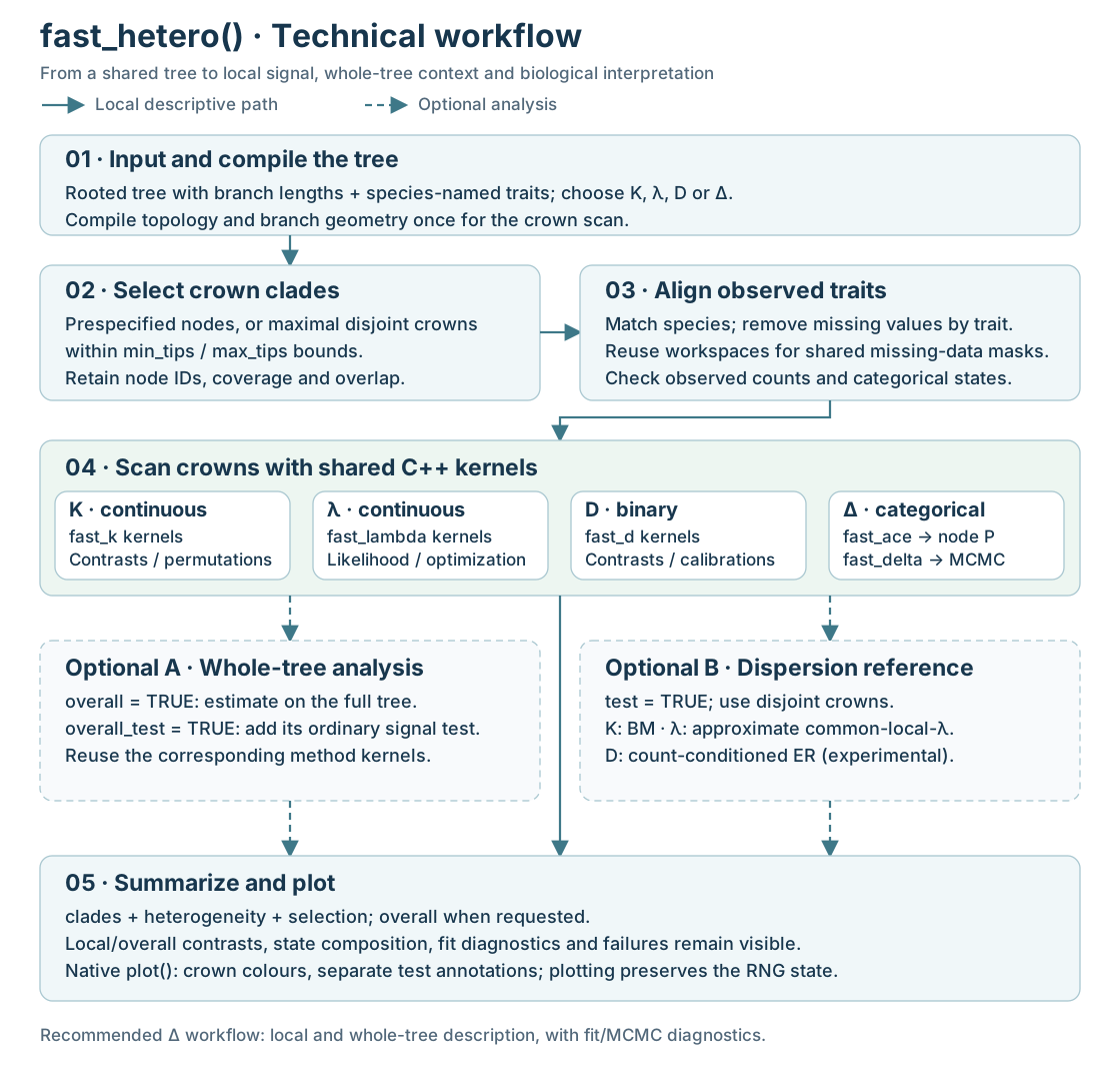
fast_hetero() compiles the tree and selects crowns, handles missing observations by trait, and reuses the C++ calculation paths for K, λ, D, ACE and Δ. Whole-tree estimates and tests are optional. Local estimates, whole-tree values, dispersion and diagnostics are then assembled in one result object.
1. Define the data design and crowns
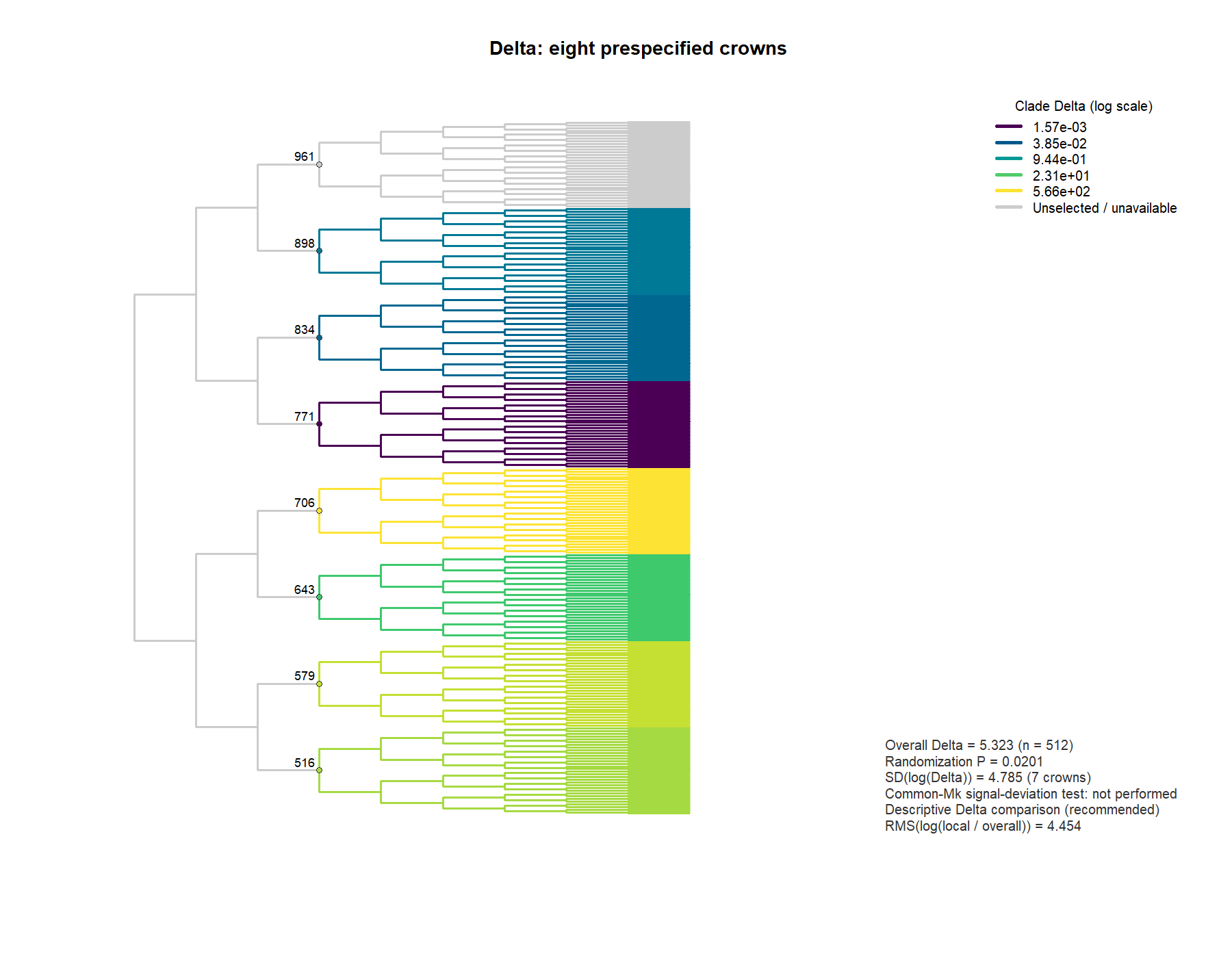
The tree is balanced, binary and ultrametric, with every branch length set to 1. Selecting nodes at root depth 3 gives eight disjoint crowns, each with 64 species and a height of 6, covering the entire tree. Selection uses the tree alone, before inspecting trait results.
Within C1–C4, continuous traits are simulated under BM and categorical traits under low-rate ER models. C5–C8 receive independent random trait values, creating a clear contrast between groups of lineages. Two common data situations are included: C1 has three missing continuous observations; C8 has only the state absent for the binary trait and A for the multistate trait.
tree <- ape::stree(512, "balanced")
tree$edge.length <- rep(1, nrow(tree$edge))
depth <- ape::node.depth.edgelength(tree)
nodes <- which(seq_along(depth) > 512 & depth == 3)
In an empirical study, specify nodes for families, genera or other biologically meaningful groups, preferably comparing crowns of similar ages and sample sizes. Without predefined groups, min_tips = 50, max_tips = 80 selects maximal disjoint crowns automatically; on this complete balanced tree it selects the same eight crowns. After choosing a primary partition, compare a small set of prespecified scales as a sensitivity analysis.
2. Continuous traits: local K and λ
Here x is a continuous trait vector named by species. Both calls use the same nodes. overall_test requests the ordinary whole-tree signal test; test requests the between-crown reference test.
k <- fast_hetero(tree, x, method = "K", nodes = nodes,
  min_tips = 50, test = TRUE, nsim = 999,
  overall_test = TRUE, progress = FALSE)

lambda <- fast_hetero(tree, x, method = "lambda", nodes = nodes,
  min_tips = 50, test = TRUE, nsim = 999,
  lambda_reference = "REML", overall_test = TRUE, progress = FALSE)

k$clades          # Observed sample sizes, local estimates, status and contrasts
k$overall         # Ordinary whole-tree signal estimates and tests
k$heterogeneity   # Between-crown dispersion and its reference test
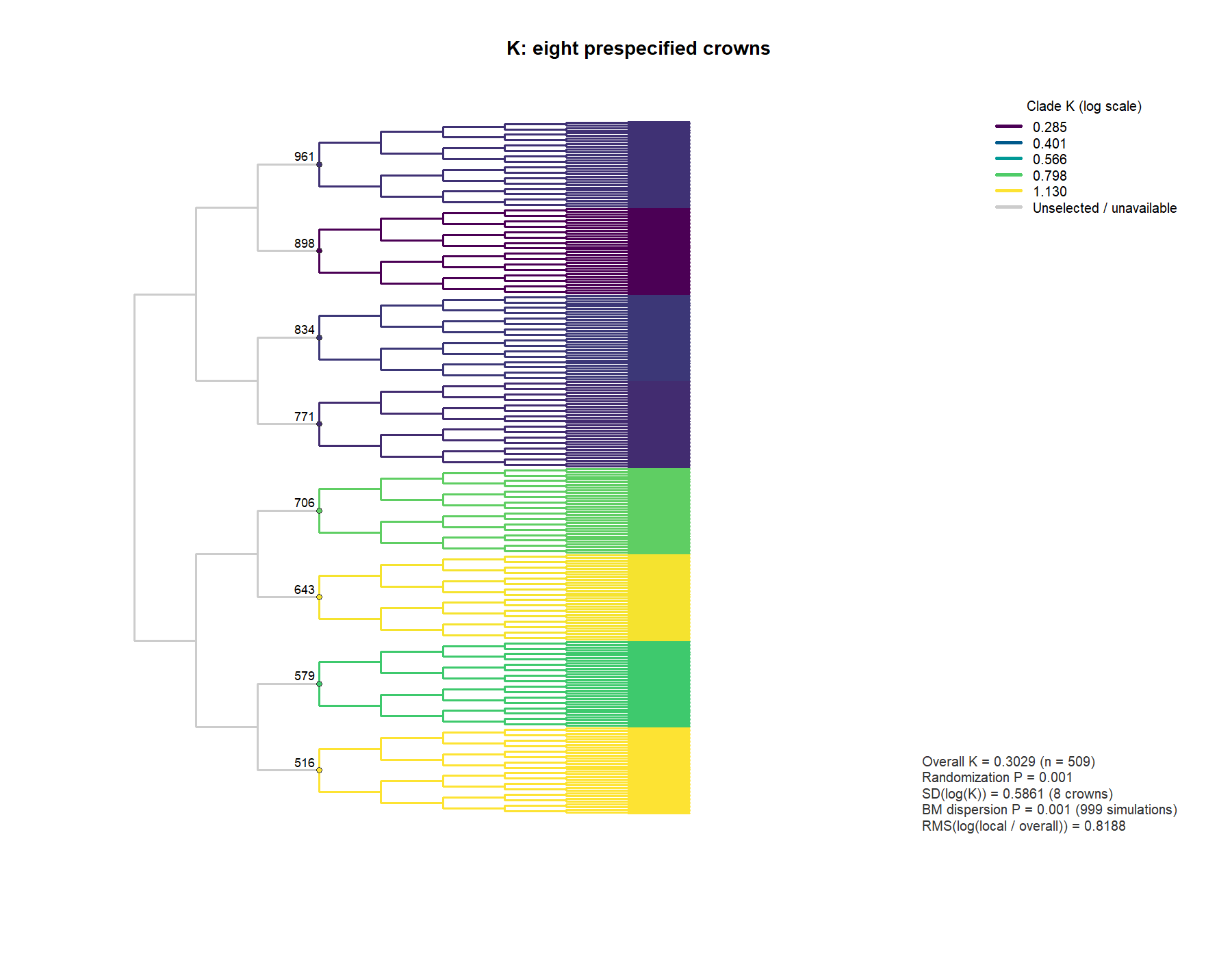
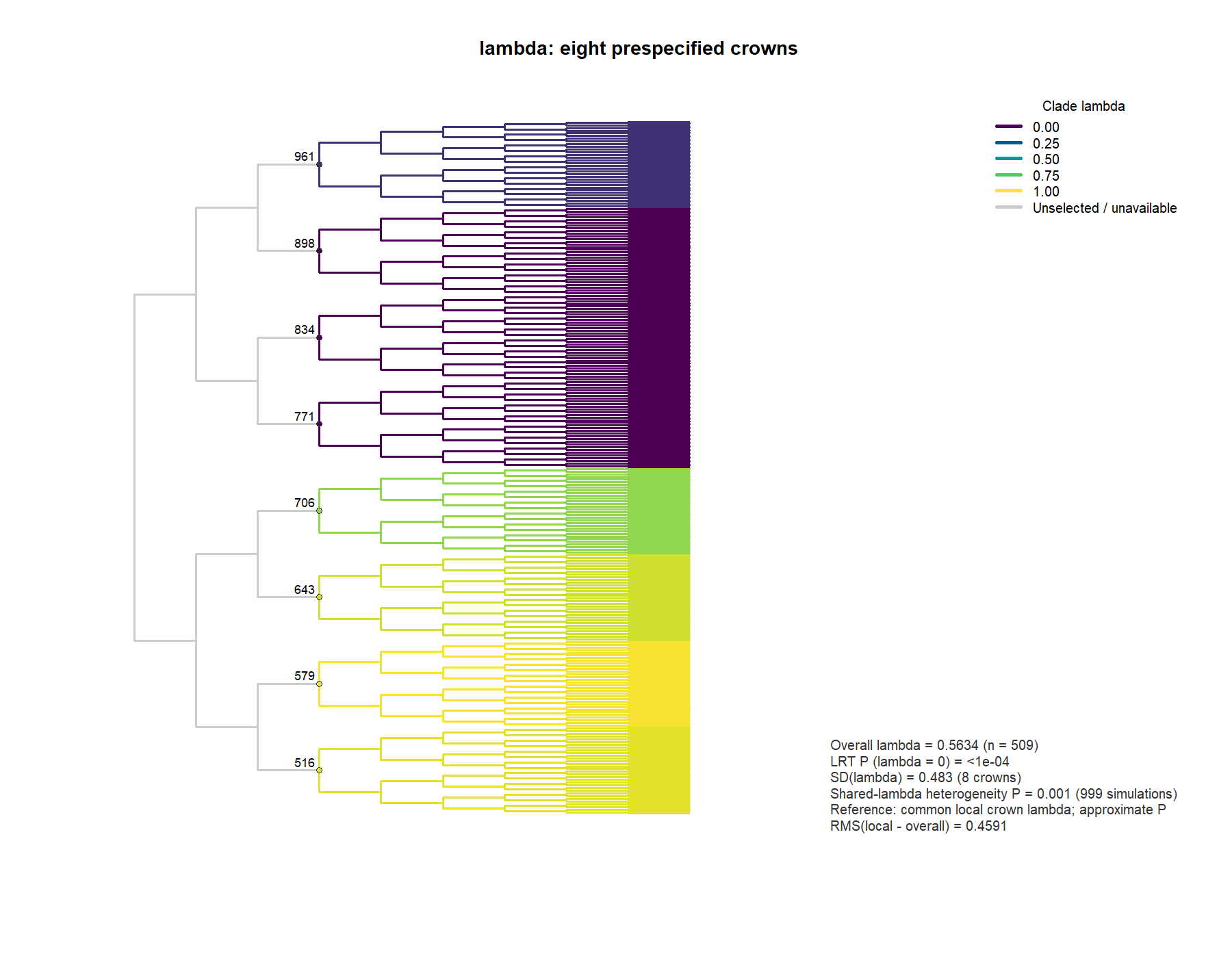
plot(k, tree = tree, show.tip.label = FALSE, node_labels = TRUE)
These are the saved outputs from the actual run. The whole-tree signal P addresses overall signal; the heterogeneity reference P asks whether between-crown dispersion exceeds the expectation under the stated reference model.
| Measure | Whole-tree estimate | Ordinary whole-tree signal P | Whole-tree n | Estimable / selected | Crown dispersion | Heterogeneity reference P |
|---|---|---|---|---|---|---|
| K | 0.3029 | 0.001001 | 509 | 8 / 8 | SD(log(K)) = 0.5861 | 0.001 |
| lambda | 0.5634 | 3.745e-17 | 509 | 8 / 8 | SD(lambda) = 0.483 | 0.001 |
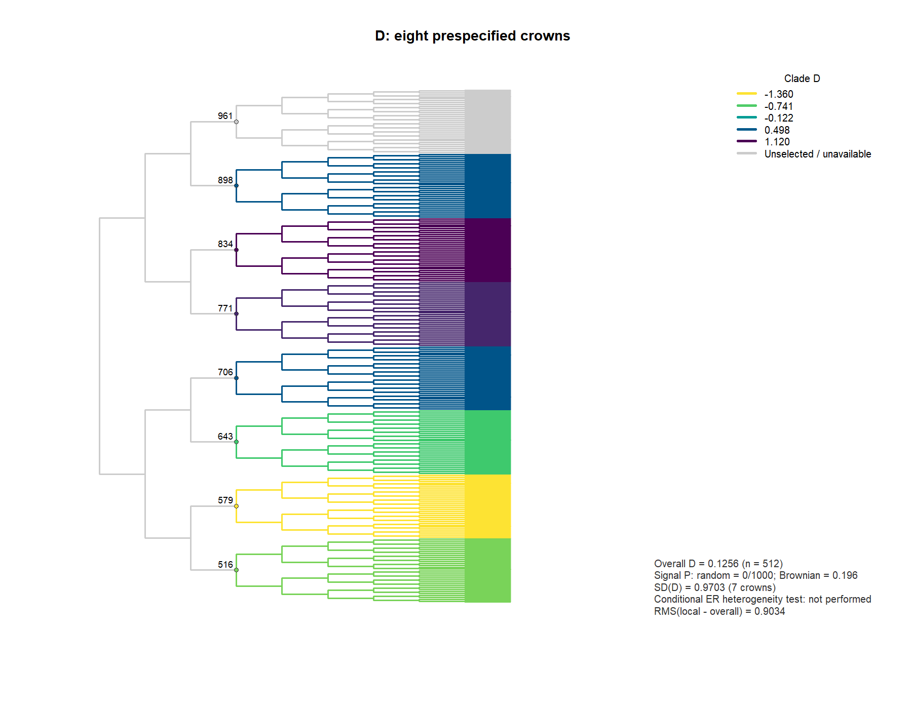
| D | 0.1256 | random: 0/1000; BM: 0.196 | 512 | 7 / 8 | SD(D) = 0.9703 | Not run (description) |
| Delta | 5.323 | 0.0201 | 512 | 7 / 8 | SD(log(Delta)) = 4.785 | Not run (description) |
The K/λ reference P of 0.001 is the +1 rank result for 999 simulations with zero exceedances, and the resolution limit of this run. The ordinary whole-tree Δ P is 4/199 = 0.0201, with MCSE about 0.00995.
K and λ both reveal lineage differences beyond the whole-tree summary. K dispersion is compared with a BM reference on the given tree; λ uses an approximate common-local-λ bootstrap. The crowns in this example have the same age, making comparison easier. In empirical data, examine crown ages too, because λ depends on the scale at which a crown is measured.
3. Categorical traits: clustering and state composition
Use D for the binary trait and Δ for the multistate trait. Both calls use test = FALSE here, so their added heterogeneity P values are not calculated. overall_test = TRUE still requests the existing ordinary whole-tree signal tests.
d <- fast_hetero(tree, binary, method = "D", nodes = nodes,
  min_tips = 51, test = FALSE, d_nsim = 1000,
  overall_test = TRUE, progress = FALSE)

delta <- fast_hetero(tree, multi, method = "Delta", nodes = nodes,
  min_tips = 50, test = FALSE, overall_test = TRUE,
  overall_nsim = 199, delta_control = list(model = "ER"),
  progress = FALSE)
Δ uses LSE and two chains of 10,000 iterations each, with burn = 100, thin = 10; ER is specified in advance. Its ordinary whole-tree test uses 199 randomizations and reports both P and Monte Carlo error. For a research analysis, choose the number of randomizations to match the probability precision needed.
| Crown | Original node | Continuous n | K | λ | D | Δ | Status |
|---|---|---|---|---|---|---|---|
| C1 | 516 | 61 | 1.125 | 0.9636 | -0.8426 | 91.24 | Estimable |
| C2 | 579 | 64 | 0.7893 | 0.9964 | -1.361 | 193.7 | Estimable |
| C3 | 643 | 64 | 1.111 | 0.9254 | -0.6767 | 19.81 | Estimable |
| C4 | 706 | 64 | 0.8178 | 0.8336 | 0.544 | 565.9 | Estimable |
| C5 | 771 | 64 | 0.3365 | 7.933e-05 | 0.8975 | 0.001573 | Estimable |
| C6 | 834 | 64 | 0.3488 | 7.933e-05 | 1.118 | 0.08829 | Estimable |
| C7 | 898 | 64 | 0.2847 | 7.933e-05 | 0.5317 | 0.1788 | Estimable |
| C8 | 961 | 64 | 0.3411 | 0.1361 | NA | NA | D/Δ single-state |
C8 remains in the results: all its categorical observations are identical, so its local D and Δ estimates are NA, with status undefined. This is a reason to examine state composition. C1 has 61 observed continuous values and the other crowns have 64; min_tips checks the count after missing observations are removed. Categorical traits have no missing values here and retain 64 species per crown.
Read each metric in its own direction: larger K, λ and Δ generally indicate stronger similarity among relatives; smaller D indicates stronger clustering, and D can fall below 0 or above 1. Compare lineages within a metric, then interpret differences alongside state composition and diagnostics.
4. Use diagnostics to interpret the pattern
| Crown | State counts | rank R-hat(Δ) | bulk ESS | tail ESS | Relative MCSE |
|---|---|---|---|---|---|
| C1 | A=50;B=2;C=12 | 1.001 | 1712 | 1682 | 0.58% |
| C2 | A=53;B=5;C=6 | 1 | 1918 | 1984 | 0.52% |
| C3 | A=40;B=7;C=17 | 0.9996 | 1812 | 1587 | 0.56% |
| C4 | A=62;B=1;C=1 | 1.001 | 1844 | 1809 | 0.80% |
| C5 | A=20;B=23;C=21 | 1.001 | 1747 | 1783 | 1.39% |
| C6 | A=17;B=27;C=20 | 0.9992 | 1925 | 1856 | 0.41% |
| C7 | A=26;B=24;C=14 | 1 | 1599 | 1865 | 0.37% |
| Whole tree | Three states | 1.003 | 1642 | 1518 | 0.17% |
The estimated Δ crowns and whole-tree result triggered no MCMC warnings in this run. The table reports rank R-hat, bulk/tail ESS and relative MCSE for the Δ sequence. The full object also retains α and β diagnostics, optimizer information, numerical recoveries and warnings. These help decide whether to extend the chains or examine rare states more closely.
A biological interpretation of this example is: “At the prespecified crown scale, C1–C4 generally show stronger similarity among relatives than the later lineages. Between-crown K dispersion exceeds the BM reference, and λ dispersion exceeds the approximate common-local-parameter reference. D and Δ show the corresponding local clustering differences for categorical traits; the single-state composition of C8 is reported separately.”
Scope. K uses a BM reference; λ uses an approximate common-local-crown reference. The added D heterogeneity test is experimental. For Δ, local/whole-tree description is recommended; heterogeneity testing is outside the recommended workflow. Signal differences describe phylogenetic conservatism at the chosen scale. Explanations involving stabilizing selection, niche conservatism or rate mechanisms require the corresponding evidence. The complete guide below documents the methods.
5. Download and reproduce the analysis
The script requires fastphylosig 0.3.4, ape and jsonlite. The data seed is 20261016, with separate fixed analysis seeds for each method. Run the downloaded script from the repository root, or set FASTPHYLOSIG_CASE_OUT to an output directory. The full script includes data generation and every parameter; the code blocks on this page are excerpts of the corresponding steps.
Download local CSVs for K, λ, D and Δ. Replace -clades.csv in a URL with -overall.csv or -heterogeneity.csv to view the corresponding full scalar table. The RDS file retains state lists and diagnostics beyond the CSV summaries.
This case was generated with the checked, frozen source package. The script also verifies that plotting preserves the random-number state. Data, saved results and session information are provided together for inspection and reuse.
Home · Install 0.3.4 · Complete statistical scope guide (Chinese)